基于注意力机制的神经机器翻译的有效方法

Effective Approaches to Attention-based Neural Machine Translation

基于注意力机制的神经机器翻译的有效方法

Bib TeX

@inproceedings{luong-etal-2015-effective, title = “Effective Approaches to Attention-based Neural Machine Translation”, author = “Luong, Thang and Pham, Hieu and Manning, Christopher D.”, booktitle = “Proceedings of the 2015 Conference on Empirical Methods in Natural Language Processing”, month = sep, year = “2015”, address = “Lisbon, Portugal”, publisher = “Association for Computational Linguistics”, url = “https://aclanthology.org/D15-1166”, doi = “10.18653/v1/D15-1166”, pages = “1412–1421”, }

abstract

在神经机器翻译中引入注意力机制(Attention)，使模型在翻译过程中选择性的关注句子中的某一部分。本文研究了两种简单有效的注意力机制。

a global approach which always attends to all source words【全局方法，每次关注所有源词】
a local one that only looks at a subset of source words at a time【局部方法，每次关注原词的一个子集】

global attention 类似方法[1]，但架构上更加简单。local attention 更像是 hard and soft attention [2]的结合。两种方法在英德语双向翻译任务中取得了不错的成绩。与已经结合了已知技术（例如 dropout）的非注意力系统相比，高了5.0个BLEU点。在WMT’15英语到德语的翻译任务中表现 SOTA（state-of-the-art）。

With local attention, we achieve a significant gain of　5.0 BLEU points over non-attentional systems that already incorporate known techniques such as dropout. Our ensemble model using different attention architectures yields a new state-of-the-art result in the WMT’15 English to German translation task with 25.9 BLEU points, an improvement of 1.0 BLEU points over the existing best system backed by NMT and an n-gram reranker.

Neural Machine Translation

模型结构：

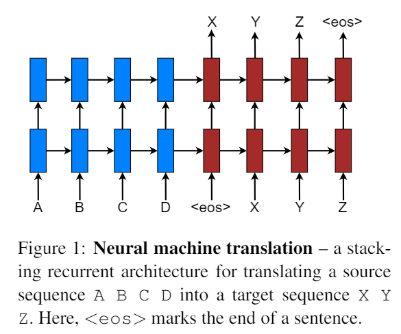
采用堆叠的 LSTM结构[3]。其目标函数为： J_t = ∑_{(x, y) ∈ D} − logP(y|x) D为训练的语料。x 表示源句子，y表示翻译后的目标句子。

Attention-based Models

这部分包括两种注意力机制：global 和 local。两种方式在解码阶段，将使用堆叠LSTM顶层的隐藏状态 h_t 作为输入。区别在于获取上下文向量表示c_t方法不同。然后通过一个简单的 concatenate layer 获得一个注意力隐藏状态ĥ_t: ĥ_t = tanh(W_c[c_t; h_t]) 最后通过 softmax layer 得出预测概率分布: p(y_t|y < t, x) = softmax(W_sĥ_t) Global Attention

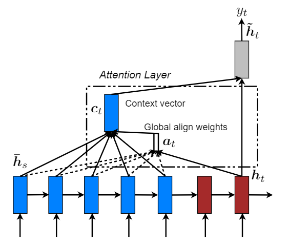
主要思想是通过编码器的所有隐藏状态(hidden state)来获取上下文向量(context vector)表示 c_t。可变长度对齐向量a_t通过比较当前目标隐藏状态h_t和每个源隐藏状态$\overline h_s$得到： $$ a_t(s) = align(h_t,\overline h_s)=\frac{exp(score(h_t,\overline h_s))}{\sum_{s'}exp(h_t,\overline h_{s^{'}})} $$ score被称为 content-based 函数： $$ score(h_t,\overline h_s)=\begin{cases} h_t^{T}\overline h_s, dot\\ h_t^{T}W_a\overline h_s, general\\ W_a[h_t;\overline h_s], concat \end{cases} $$ 与[1]的区别在于：

只在编码器和解码器的顶部使用隐藏状态
计算路径更加简单：h_t− > a_t− > c_t− > ĥ_t

Local Attention

global 模式下，模型需要关注全局信息，其代价是非常大的。因此也就出现了 local attention。让注意力机制只去关注其中的一个子集部分。其灵感来自于 [2]。

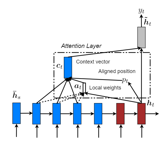
对比两张模型图来看，其中的局部对齐权重a_t由一部分局部隐藏状态计算得到，其长度变成了固定的，并且还多了一个Aligned position p_t ，然后上下文向量(context vector) c_t 由窗口[p_t − D, p_t + D]内的隐藏状态集合的加权平均得到。其中D根据经验所得。

考虑两种变体：

Monotonic alignment (local-m)

即简单设置 p_t = t ，认为源序列于目标序列是单调对齐的，那么a_t 其实就和公式（4）计算方法一样了。
Predictive alignment (local-p)

p_t = S · sigmoid(v_p^Ttanh(W_ph_t)) ，v_p和W_p是预测p_t 的模型参数。S为源句子长度。最后p_t ∈ [0, S] 。同时为了使对齐点更靠近p_t，设置一个以p_t为中心的高斯分布，即a_t 为：$a_t(s)=align(h_t,\overline h_s)exp(-\frac{(s-p_t)^2}{2\sigma^2}),\sigma=\frac{D}{2}$，s为高斯分布区间内的一个整数。

Input-feeding Approach

这一部分，主要是为了捕获在翻译过程中哪些源单词已经被翻译过了。对齐决策应当综合考虑过去对齐的信息。该方法将注意力向量ĥ_t 作为下一个时间步的输入。主要有两个作用：

希望模型充分关注到先前的对齐信息
创建一个在水平和垂直方向上都很深的网络

总结

整篇论文看下来，大概就是在别人的baseline中引入注意力机制（global and local），然后使用Input-feeding 方法将过去的对齐信息考虑进来（大概就是加入了一个先验知识吧）。【PS：震惊！这些创新的点的灵感都来自其让人的论文中的方法。】

最后手动滑稽：

Attention is all you need!

References

[1] Dzmitry Bahdanau, Kyunghyun Cho, and Yoshua Bengio. 2015. Neural machine translation by jointly learning to align and translate. InICLR.

[2] Kelvin Xu, Jimmy Ba, Ryan Kiros, Kyunghyun Cho, Aaron C. Courville, Ruslan Salakhutdinov, Richard S. Zemel, and Yoshua Bengio. 2015. Show,attend and tell: Neural image caption generation with visual attention. InICML.

[3] Wojciech Zaremba, Ilya Sutskever, and Oriol Vinyals. 2015. Recurrent neural network regularization. InICLR.